Blog Details

This blog is part of our pgvector blog series. If you haven’t checked out the first blog, I recommend going through it first, where I dive into important concepts of pgvector and AI applications in detail. I provided a real-world example illustrating how you can perform searches based on the meaning of words rather than the words themselves. You can find it on the link here

In this blog, We will explore additional details about the indexes supported in pgvector. We will discuss how indexes are built in the backend, and the various parameters associated with these indexes, and guide you on selecting the most suitable index based on your requirements. Finally, we will assess which index offers the best recall rate for our search query across our dataset of one million records sourced from Wikipedia. Let’s dive into that

pgvector supports 2 types of indexes Inverted File(IVFFLAT) and Hierarchical Navigable Small World(HNSW) both are Approximate Nearest Neighbor(ANN) indexes means they can efficiently search nearby neighbors that are close enough to the query vector

Note: To create an index on a full column, the column must have a consistent number of vector dimensions across all its rows. For instance, if a table named country has a vector column named city, and one row in this city column consists of 1536 dimensions of vector data while the next row consists of only 500 dimensions, we won’t be able to create a full index on that column. If dimensions vary, consider creating partial indexes

IVFFLAT

This was the first index introduced in pgvector. When we generate an IVFFLAT index, it finds similar-looking vectors and forms multiple clusters, It then calculates a central point for each cluster, known as a centroid. Each vector is then assigned to its nearest centroid. This clustering ensures that during similarity searches, we only look for vectors close to the query vector, excluding less similar ones. And can improve search speed. The diagram below shows how a centroid is formed and how similar-looking vectors are assigned to one region

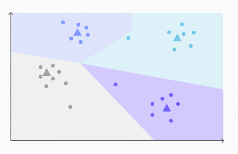
Source: Timescale

Build IVFFLAT when data is substantial

We can only create the IVFFLAT index once we have a sufficient amount of data inside the table this is because of a few reasons

• The clustering algorithm used in IVFFLAT relies on having enough data points to accurately capture the underlying data distribution and form meaningful clusters.
• Centroids, the representative points of each cluster, are calculated based on the data points within the cluster.
• The inverted file, which maps centroids to vectors within each cluster, is more effective when the clusters accurately reflect data similarity.

While there’s no strict threshold for sufficient data, it’s generally recommended to have at least several thousand data points before building an IVFFLAT index to ensure meaningful clustering, accurate centroids, and effective performance.

Use the following query to create the index

CREATE INDEX ON <TABLE_NAME> USING ivfflat (<COL_NAME> <SIMILARITY_SEARCH_METHOD>) WITH (lists = <NUMBER_OF_LISTS>);

In the above query, the list determines how many clusters we want to create while building the index. More lists lead to faster searches by narrowing down potential matches quickly. However, too many lists can negatively impact recall, as exploring fewer sub-groups might miss relevant neighbors

The recommended value for selecting the list is 

• rows / 1000 for up to 1M rows i.e if you have 1Million rows inside the table then the value of the list would be 1000
• sqrt(rows) for over 1M rows i.e, if you have 2Million rows inside the table then lists value should be 1415

A similarity search method can be 

• Vector_l2_ops
• Vector_ip_ops
• Vector_cosine_ops

Unfamiliar? Check our previous blog here for detailed explanations

Caution: Building the index

We also need to keep maintenance_work_mem in account while building the index because building the index involves memory-intensive operations like distance calculations and data comparisons. So it is better we allocate a sufficient amount of maintenance_work_mem before starting to create the indexes there is no such rule or recommendation for value for maintenance_work_mem a good starting point can be 

• For smaller Datasets (up to a few million vectors): 512MB to 1GB often suffices.
• For larger Datasets (tens of millions or more): 2GB to 4GB or even higher might be necessary
• We can also consider temporarily increasing maintenance_work_mem for index building, then decreasing it. Alternatively, set it at the session level.

pgvector provides hints on memory requirements for efficient index creation. For instance, attempting to create an index on 1 million rows with default 64MB maintenance_work_mem triggered the following error for me

ERROR: memory required is 501 MB, maintenance_work_mem is 64 MB

Potential performance issue with IVFFLAT

IVFFLAT is an approximate nearest neighbor (ANN) algorithm, that focuses on speed rather than exactness in identifying nearest neighbors. During a search process, it begins by identifying the closest cluster centroid(s) to the query point. However, this approach may overlook relevant vectors that lie just outside those clusters or are closer to the query point than their respective cluster centroid. As a result, while IVFFLAT offers fast search capabilities, there is a trade-off in terms of potentially missing some of the exact similar vectors.

Probes

Probes tackle this challenge by enabling IVFFLAT to explore a broader range of clusters or regions, enhancing the chances of discovering the actual nearest neighbors. By specifying additional probes, we can extend our search across more regions, enhancing search quality and reducing the risk of overlooking the true closest vector. It’s important to note that while employing more probes may improve accuracy by examining additional clusters, it also comes with the trade-off of increased search time.

The recommended value for probes is sqrt(lists) i.e, if you have 1000 lists then probes should be 31

SET ivfflat.probes = 32;

By default, its value is 1 which means it will only search inside the closest centroid cluster/rigion and will not consider other regions

Rebuilding the index

IVFFLAT’s structure heavily relies on the initial dataset distribution. It calculates clustering, lists, centroids, and data points initially. But in the real world when data is added, updated, or deleted, the index may become fragmented and can cause slower search speeds, higher memory usage, and less accurate results so rebuilding the index allows it to re-cluster and regenerate the inverted file based on the updated data, optimizing search accuracy and performance

It is always a good idea to rebuild the index 

• After major additions, removals, or shifts in data distribution. So frequent changes might need more frequent rebuilding
• When search speed or accuracy is noticeably decreasing
• For large datasets, consider periodic rebuilding even without obvious issues

Note: We need to be careful of any ongoing database operations that might be affected by the rebuild process.

Use the following query to rebuild the index

REINDEX INDEX <INDEX_NAME>;

Searching via IVFFLAT index

When a search vector appeared

• We initially compute the distance between the query vector and all the centroids. 
• After identifying the nearest centroid, we then assess the distance between the query vector and each vector linked to this selected centroid. 
• Ultimately, we choose the vector with the closest distance as the resulting vector. 

Ensuring the selection of the most similar vector as the outcome.

When to use the IVFFLAT index

Consider using the IVFFLAT index when:

• It’s okay to tolerate a slight decrease in search accuracy.
• There are no strict limitations on memory.
• Data updates don’t happen too often.
• If you want the index to be built quickly and take up less space.

HNSW

Launched in pgvector 0.5.0, this index type stands out for its notable features, It has better query performance than the IVFFLAT index, but builds slower and uses more memory. Unlike IVFFLAT, creating the index doesn’t require a training step. You can create it immediately after setting up the relation/table, even if it’s empty.

HNSW index built using concepts from skiplists and Navigable Small World Graphs to achieve efficient ANN search in high-dimensional spaces

SkipList

A skiplist is a probabilistic data structure that aims to improve the search performance of a traditional linked list by introducing multiple levels of access (or “skips”). Imagine flipping through a large phonebook – a traditional linked list would require reading every name in order, while a skip list provides shortcuts at certain intervals to speed up the search.

• Each element in the list is a node containing a value and links to other nodes.
• Nodes at different levels are connected vertically through additional “skip” pointers.
• The bottom level is a traditional single-dimensional linked list where all nodes are connected sequentially.
• Higher levels have fewer nodes, with each node skipping over a certain number of nodes in the level below.

Source: Supabase

How search works in skiplist

We begin the search at the top level of the Skip List,

• We compare the target element with the next element in the current level.
• If the next element is less than the target element, move forward to the next element in the same level. If the next element is greater than the target element, move down to the next level and repeat step 2.
• Continue moving forward or down until the target element is found or until reaching the end of the Skip List.
• If the target element is found, return the element or its location. If the target element is not found, return an indication that the element is not in the Skip List.

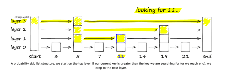
Source: Pinecone

Check this Wikipedia article to learn more about skip lists: https://en.wikipedia.org/wiki/Skip_list

Navigable Small World Graphs

The Navigable Small World Graph (NSWG) is a graph structure where each vertex is connected to several other vertices, forming a friend list. During a search in an NSWG, we start at an entry point connected to nearby vertices and move to the closest one iteratively through greedy-routing. This process continues until we reach a local minimum, indicating no nearer vertices are available. 

HNSW – A Combination of skiplists and Navigable Small World Graphs

HNSW combines concepts from skiplists and Navigable Small World Graphs (NSW) to create a powerful algorithm for efficient nearest-neighbor search. At its core, HNSW uses a Navigable Small World Graph structure, ensuring that nodes in the network maintain both local clustering and short path lengths. This means that similar data points are closely connected, facilitating quick searches within local neighborhoods. Each layer represents a different level of granularity in the data, allowing for more effective navigation during the search process. Like the layers in a skiplist, these hierarchical levels provide shortcuts, enabling the algorithm to skip unnecessary comparisons and converge faster to the nearest neighbors.

In the below diagram, we can see a hierarchical structure that forms an inverted tree. The uppermost layer consists of a carefully chosen subset of data points, often referred to as entry points. As we move down through the layers, the number of data points increases, and the bottom layer contains all the data points in the dataset. Each layer is connected not only vertically to the layers above or below but also horizontally to the same level, creating a multi-layered graph structure. This network of connections makes efficient navigation and searching of the dataset, and allowing the algorithm to create a balance between local and global searches for nearest neighbors.

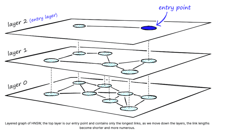
Source: Pinecone

Note: The IVFFLAT index should be created once you have a sufficient amount of data inside the table. Whereas an HNSW index can be built even if the table is empty. This is mainly because HNSW does not require a training step, unlike IVFFLAT.

How search works in HNSW index

During a search, the algorithm traverses this graph by starting from the top level. The algorithm compares your query vector to the neighbors of the current node based on a chosen distance metric (e.g., cosine similarity). If the exploration gets stuck in a local minimum (not finding significantly closer neighbors), the algorithm will switch to a lower layer in the hierarchy. Once reaching the bottom layer (highest detail), the algorithm continues exploring neighbors until it finds the desired nearest neighbor vector based on your query. The data points (corresponding to nodes) identified as nearest neighbors are returned as the search results.

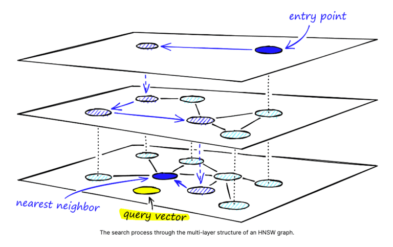
Source: Pinecone

To create HNSW index use the following query:

CREATE INDEX ON items USING hnsw (embedding vector_l2_ops) WITH (m = 16, ef_construction = 64);

M

The parameter M in the HNSW graph specifies the maximum number of connections that each vertex/node has with its nearest neighbors. It influences the graph’s connectivity, with higher values indicating denser connections. A higher M allows for faster graph exploration, potentially leading to quicker searches. However, it may also increase the likelihood of missing relevant neighbors who are further away. Conversely, a lower M reduces exploration options, potentially slowing down searches, especially when reaching distant neighbors. Lower M values may improve accuracy (recall) by forcing the search to explore a wider range, increasing the chances of finding relevant neighbors.

ef_construction

This parameter defines the maximum number of candidates the algorithm considers when adding a new data point to the graph. Higher values consider more potential related neighbors during construction, potentially resulting in a more accurate and well-connected graph. However, evaluating more candidates takes more time, leading to longer index creation. Lower values lead to faster index build time as less evaluation work is required. However, this may result in lower index quality as fewer candidates are explored, potentially impacting search performance.

ef_search

This parameter defines the maximum number of candidate neighbors the search algorithm will consider during a search operation in an HNSW index. Higher values can result in slower searches due to the evaluation of more candidates, leading to potentially more comparisons and slower search times. However, they offer higher recall by exploring more neighbors, increasing the chances of finding relevant ones, even if they are not the absolute closest. Conversely, lower values can lead to faster searches by evaluating fewer candidates, potentially resulting in quicker search times. However, they may also result in lower recall due to less exploration, potentially missing some relevant neighbors and impacting recall.

SET hnsw.ef_search = 100; -- by default its value is 40

When to use the HNSW index

Consider using the HNSW index when:

• When you need high recall speed
• If data is rapidly changing
• If you want to store high-dimensional data
• Recall accuracy can be tolerate 

Testing recall speed of indexes

Let us now dive into the example and see what performance improvement we can get by using indexes in pgvector 

We created 3 tables 

• Table without any index: demo_table
• Table with IVFFLAT index: wiki_data_ivf 
• Table with HNSW index: wiki_data
• pgvector version: 0.6.0
• PostgreSQL version: 16.1

and populated them with the same data set from dbpedia-entities-openai-1M

We are running EXPLAIN and ANALYSE on a query by selecting text and cosine distance from the table where the difference with ‘<EMB>’ is over 0.8 and selecting only 1 row.

EXPLAIN ANALYSE SELECT text, (openai <=> '<EMB>') AS cosine_distance FROM demo_table WHERE 1 - (openai <=> '<EMB>') > 0.8 ORDER BY cosine_distance ASC LIMIT 1;

Recall Without index

Parallel Seq Scan on demo_table  (cost=0.00..61781.66 rows=138867 width=339) (actual time=33.277..4119.286 rows=41 loops=3)
Planning Time: 1.982 ms
Execution Time: 4145.951 ms

Recall with IVFFLAT index

Index Scan using wiki_table_ivf_openai_idx on wiki_table_ivf  (cost=2512.50..7327.33 rows=333333 width=340) (actual time=12.434..12.434 rows=1 loops=1)
Planning Time: 1.005 ms
Execution Time: 12.491 ms

Recall with HNSW index

Index Scan using wiki_table_openai_idx on wiki_table  (cost=384.72..2063911.53 rows=333433 width=340) (actual time=8.548..8.549 rows=1 loops=1)
Planning Time: 0.937 ms
Execution Time: 8.642 ms

We observe a significant improvement from an initial time of 4 to 5 seconds, reduced to just 12 ms with the IVFFLAT index. Furthermore, the search time was further reduced to just 8.6 ms with the HNSW index.